3. Results
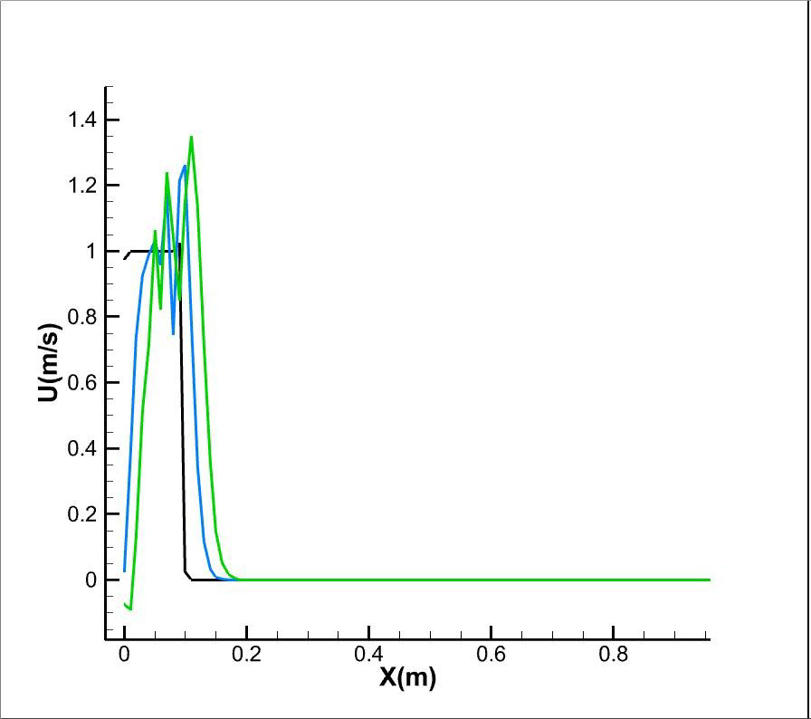
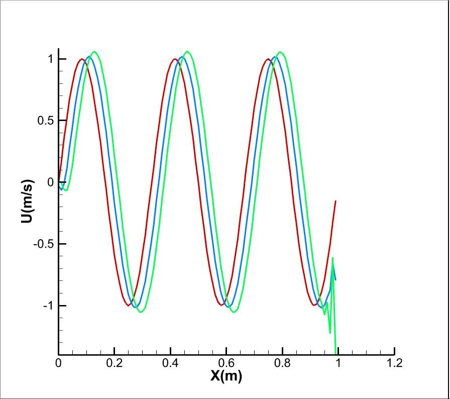
Figure 1:
First-order Crank-Nicolson & Second-order Crank-Nicolson
In the Crank-Nicholson method, by increasing the spatial and temporal steps while keeping the Courant number constant, the amount of numerical error increases. The results for this method can be found in the corresponding folder, but it was not possible to plot it here. The three-dimensional matrix solver function has been tested for specific problems, and no errors have been observed in the solver code.
In Short:
- Decreasing the Courant number in the initial time steps provides results closer to the exact solution.
- Increasing the number of nodes at a fixed Courant number increases accuracy in methods with fewer calculation steps.
- As the time step increases, dispersion and propagation errors increase, leading to a deviation from the exact solution.